Predict availability in #TidyTuesday water sources with random forest models
By Julia Silge in rstats tidymodels
May 6, 2021
This is the latest in my series of
screencasts demonstrating how to use the
tidymodels packages, from just starting out to tuning more complex models with many hyperparameters. Today’s screencast walks through how to train and evalute a random forest model, with this week’s
#TidyTuesday dataset on water sources. 🚰
Here is the code I used in the video, for those who prefer reading instead of or in addition to video.
Explore data
Our modeling goal is to predict whether a water source actually has water available at it, based on characteristics of the water source observed during a visit. Let’s start by reading in the data.
library(tidyverse)
water_raw <- read_csv("https://raw.githubusercontent.com/rfordatascience/tidytuesday/master/data/2021/2021-05-04/water.csv")
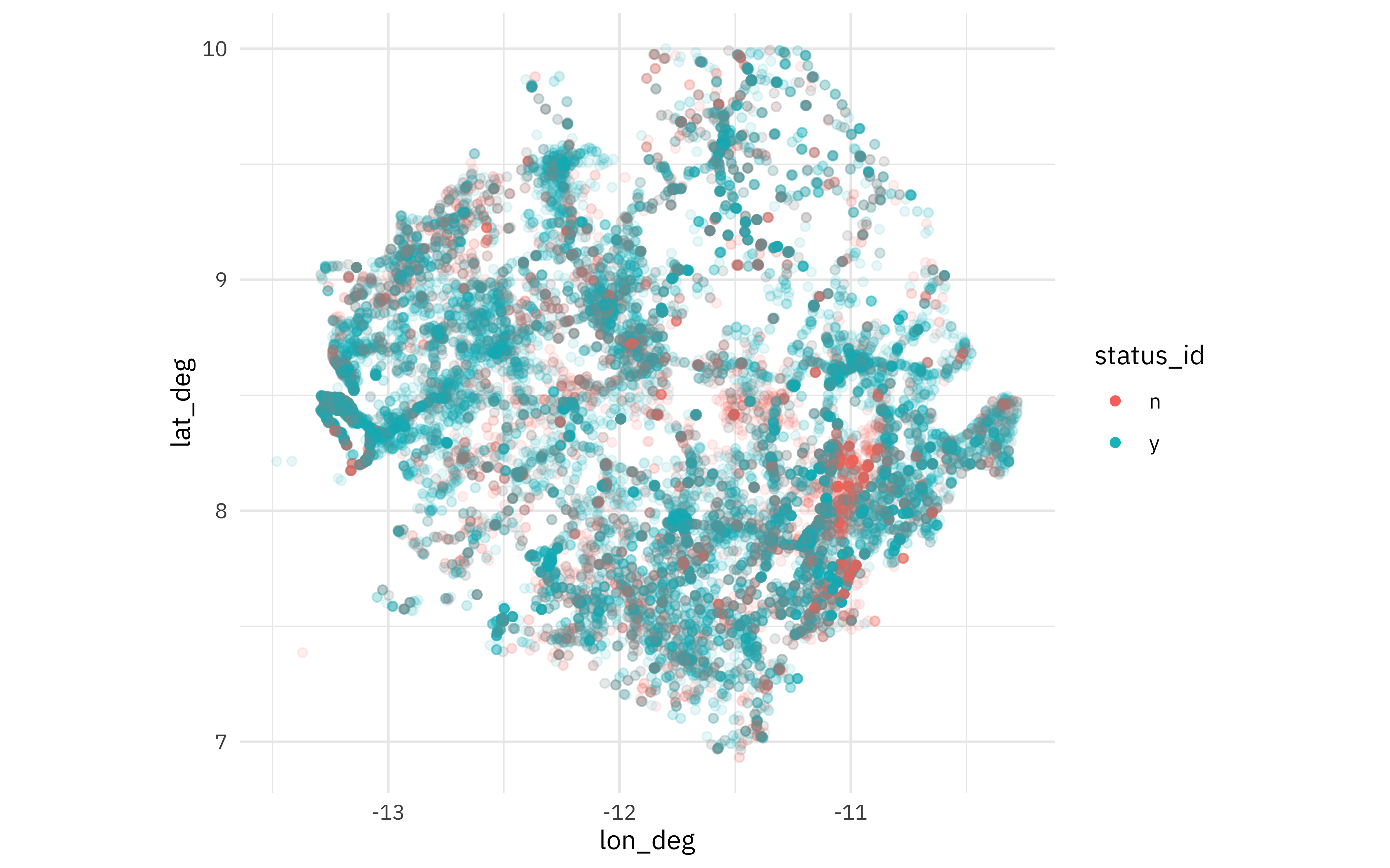
Let’s restrict this model analysis to only water sources in Sierra Leone, and just the water sources that were cataloged as “y” or “n” for water availability. How are these water sources distributed across Sierra Leone?
water_raw %>%
  filter(
    country_name == "Sierra Leone",
    lat_deg > 0, lat_deg < 15, lon_deg < 0,
    status_id %in% c("y", "n")
  ) %>%
  ggplot(aes(lon_deg, lat_deg, color = status_id)) +
  geom_point(alpha = 0.1) +
  coord_fixed() +
  guides(color = guide_legend(override.aes = list(alpha = 1)))
Let’s create a new water data set to use moving forward, and handle the pay variable.
water <- water_raw %>%
  filter(
    country_name == "Sierra Leone",
    lat_deg > 0, lat_deg < 15, lon_deg < 0,
    status_id %in% c("y", "n")
  ) %>%
  mutate(pay = case_when(
    str_detect(pay, "^No") ~ "no",
    str_detect(pay, "^Yes") ~ "yes",
    is.na(pay) ~ pay,
    TRUE ~ "it's complicated"
  )) %>%
  select(-country_name, -status, -report_date) %>%
  mutate_if(is.character, as.factor)
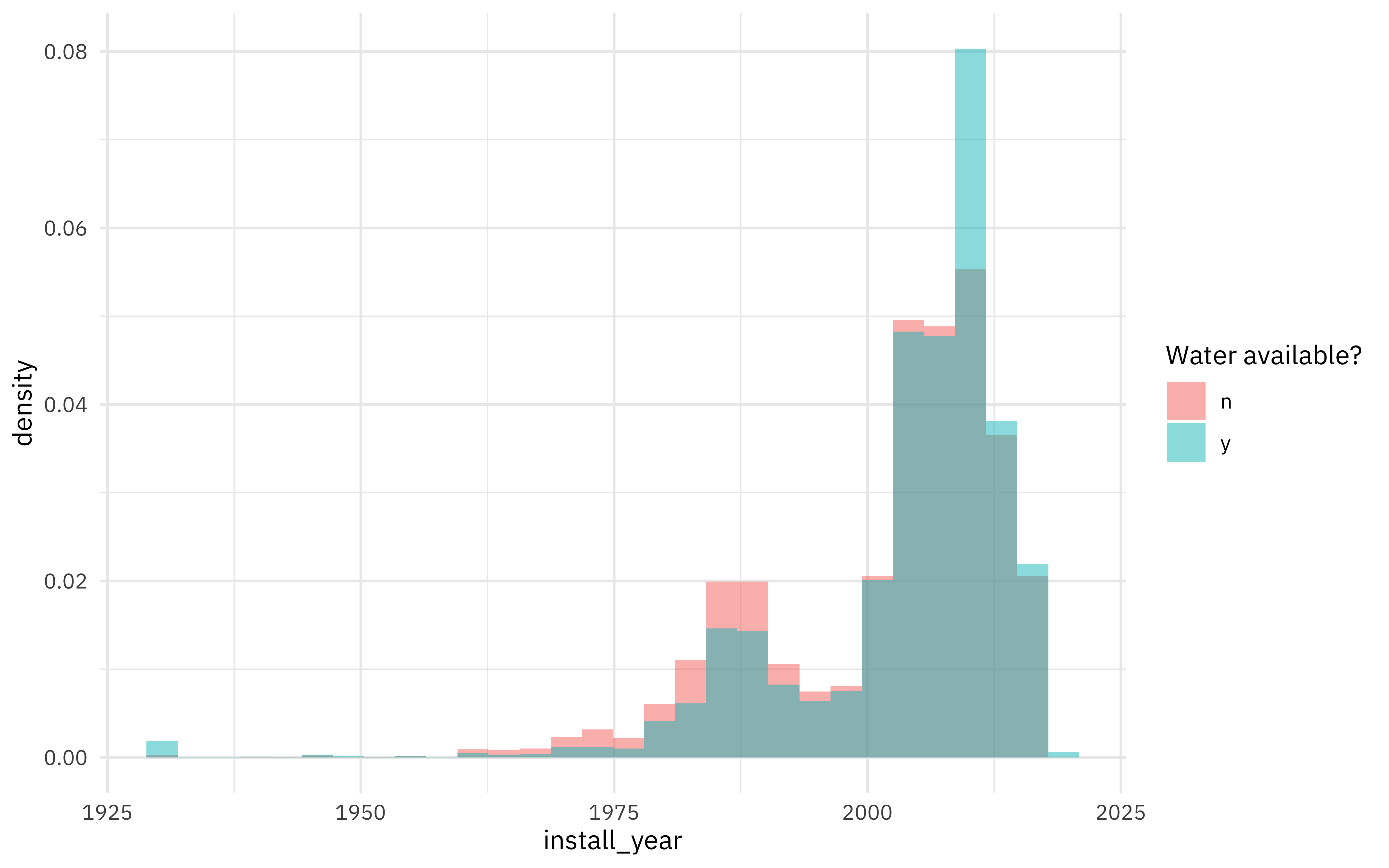
Do we see differences in water availability by when a source was installed?
water %>%
  ggplot(aes(install_year, y = ..density.., fill = status_id)) +
  geom_histogram(position = "identity", alpha = 0.5) +
  labs(fill = "Water available?")
What about by payment status of the water source?
water %>%
  ggplot(aes(y = pay, fill = status_id)) +
  geom_bar(position = "fill") +
  labs(fill = "Water available?")
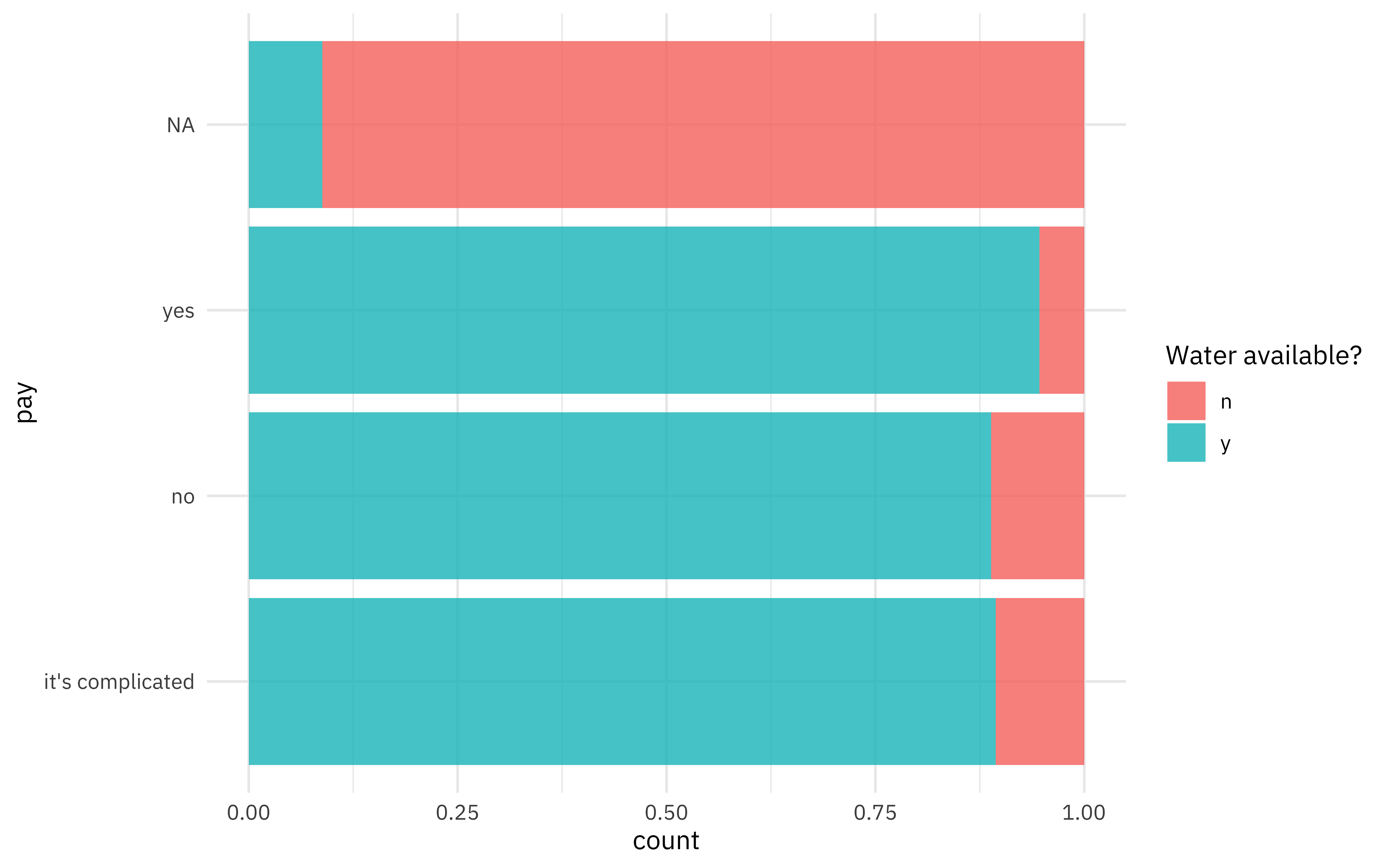
This may be an issue with the data itself; we may not have as much information about payment for water sources that didn’t have water available at the time of the visit. This would definitely be worth learning more!
Build a model
Let’s start our modeling by setting up our “data budget.”
library(tidymodels)

set.seed(123)
water_split <- initial_split(water, strata = status_id)
water_train <- training(water_split)
water_test <- testing(water_split)

set.seed(234)
water_folds <- vfold_cv(water_train, strata = status_id)
water_folds
## #  10-fold cross-validation using stratification
## # A tibble: 10 x 2
##    splits               id
##    <list>               <chr>
##  1 <split [36985/4110]> Fold01
##  2 <split [36985/4110]> Fold02
##  3 <split [36985/4110]> Fold03
##  4 <split [36985/4110]> Fold04
##  5 <split [36985/4110]> Fold05
##  6 <split [36986/4109]> Fold06
##  7 <split [36986/4109]> Fold07
##  8 <split [36986/4109]> Fold08
##  9 <split [36986/4109]> Fold09
## 10 <split [36986/4109]> Fold10
For this analysis, I used the usemodels package to set up my modeling code quickly.
usemodels::use_ranger(status_id ~ ., data = water_train)
This generated code for me that I could then go in and edit. I especially needed to add to the feature engineeering part of my modeling code.
library(themis)
ranger_recipe <-
  recipe(formula = status_id ~ ., data = water_train) %>%
  update_role(row_id, new_role = "id") %>%
  step_unknown(all_nominal_predictors()) %>%
  step_other(all_nominal_predictors(), threshold = 0.03) %>%
  step_impute_linear(install_year) %>%
  step_downsample(status_id)

ranger_spec <-
  rand_forest(trees = 1000) %>%
  set_mode("classification") %>%
  set_engine("ranger")

ranger_workflow <-
  workflow() %>%
  add_recipe(ranger_recipe) %>%
  add_model(ranger_spec)

doParallel::registerDoParallel()
set.seed(74403)
ranger_rs <-
  fit_resamples(ranger_workflow,
    resamples = water_folds,
    control = control_resamples(save_pred = TRUE)
  )
Modeling done! I chose not to tune the random forest because they typically do pretty well if you give them enough trees.
Explore results
How did the random forest models perform?
collect_metrics(ranger_rs)
## # A tibble: 2 x 6
##   .metric  .estimator  mean     n std_err .config
##   <chr>    <chr>      <dbl> <int>   <dbl> <chr>
## 1 accuracy binary     0.893    10 0.00179 Preprocessor1_Model1
## 2 roc_auc  binary     0.951    10 0.00145 Preprocessor1_Model1
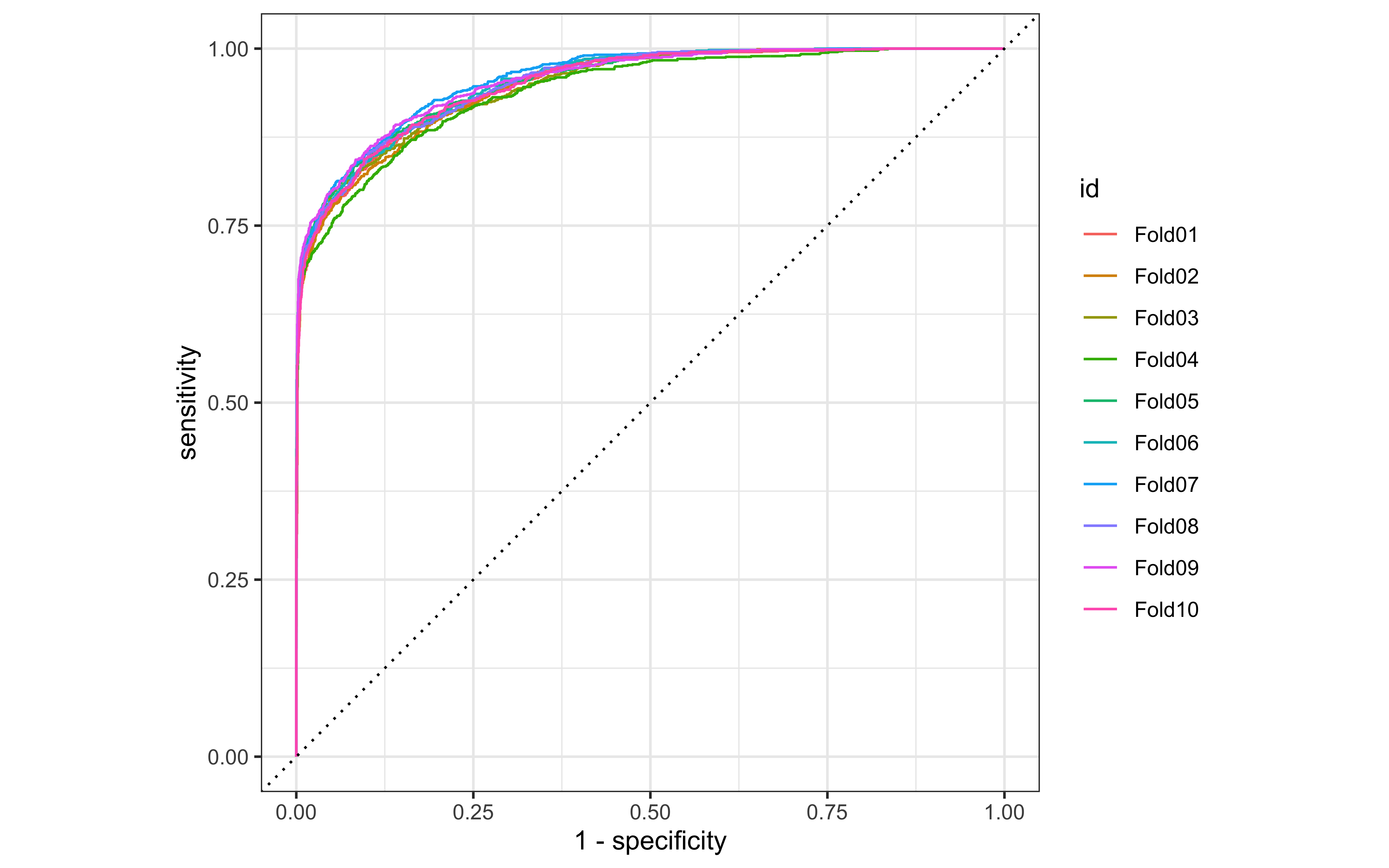
We can look at ROC curves for the set of 10 cross-validation folds.
collect_predictions(ranger_rs) %>%
  group_by(id) %>%
  roc_curve(status_id, .pred_n) %>%
  autoplot()
We can also create a confusion matrix from the resamples using conf_mat_resampled().
conf_mat_resampled(ranger_rs, tidy = FALSE) %>%
  autoplot()
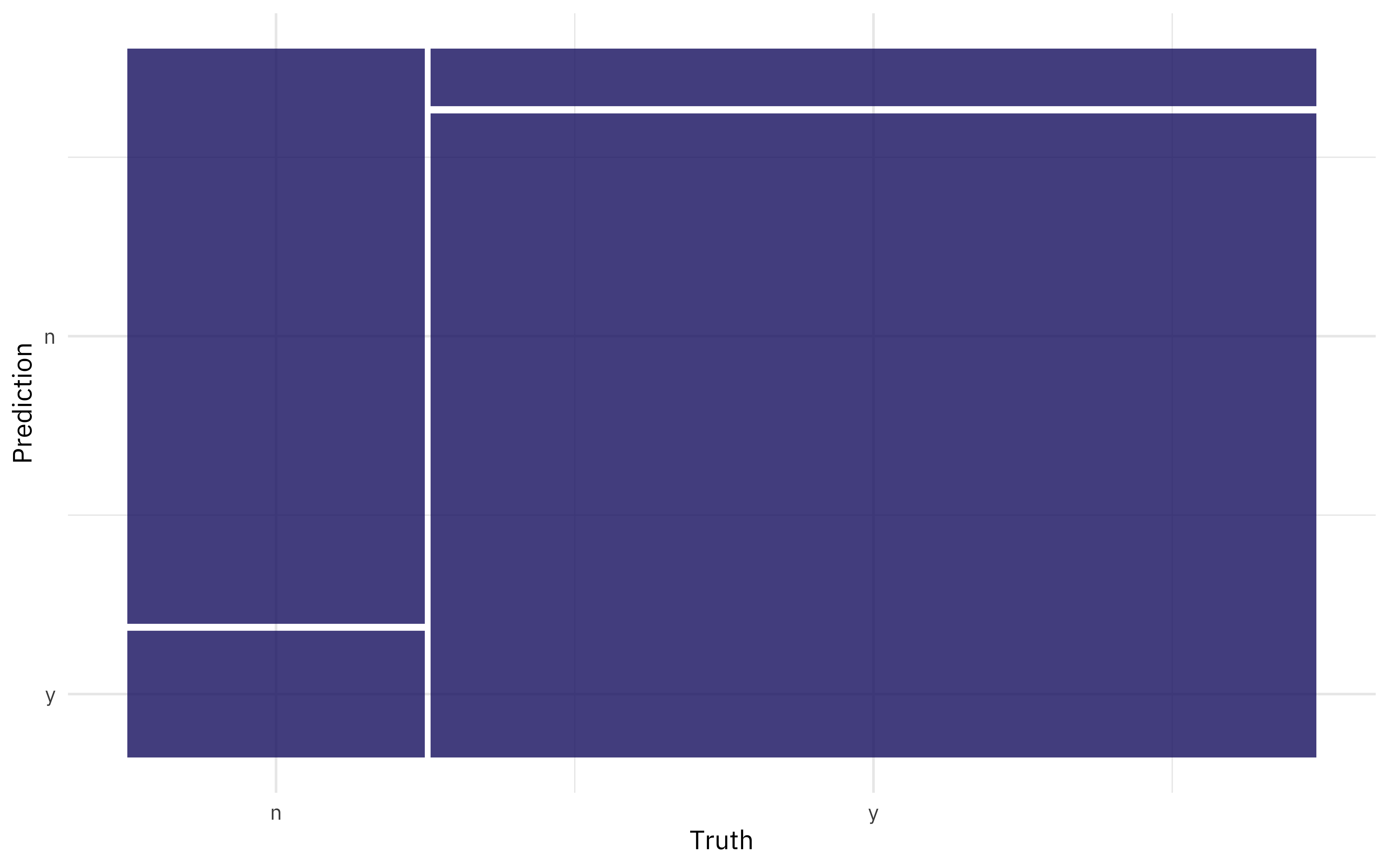
These results look pretty good (with the caveat about the pay feature) so let’s fit one final time to the entire training set at once and evaluate once on the test set. This is the first time we have used the test set.
final_fitted <- last_fit(ranger_workflow, water_split)
collect_metrics(final_fitted) ## metrics on the *testing* set
## # A tibble: 2 x 4
##   .metric  .estimator .estimate .config
##   <chr>    <chr>          <dbl> <chr>
## 1 accuracy binary         0.892 Preprocessor1_Model1
## 2 roc_auc  binary         0.951 Preprocessor1_Model1
We can collect predictions on the testing set and create an ROC curve or, as shown here, a confusion matrix.
collect_predictions(final_fitted) %>%
  conf_mat(status_id, .pred_class) %>%
  autoplot()

What about variable importance? Let’s use the
vip package to computer variable importance for this random forest; we’ll have to fit the model again using importance = "permutation" and a data set imp_data that we preprocessed manually.
library(vip)

imp_data <- ranger_recipe %>%
  prep() %>%
  bake(new_data = NULL) %>%
  select(-row_id)

ranger_spec %>%
  set_engine("ranger", importance = "permutation") %>%
  fit(status_id ~ ., data = imp_data) %>%
  vip(geom = "point")
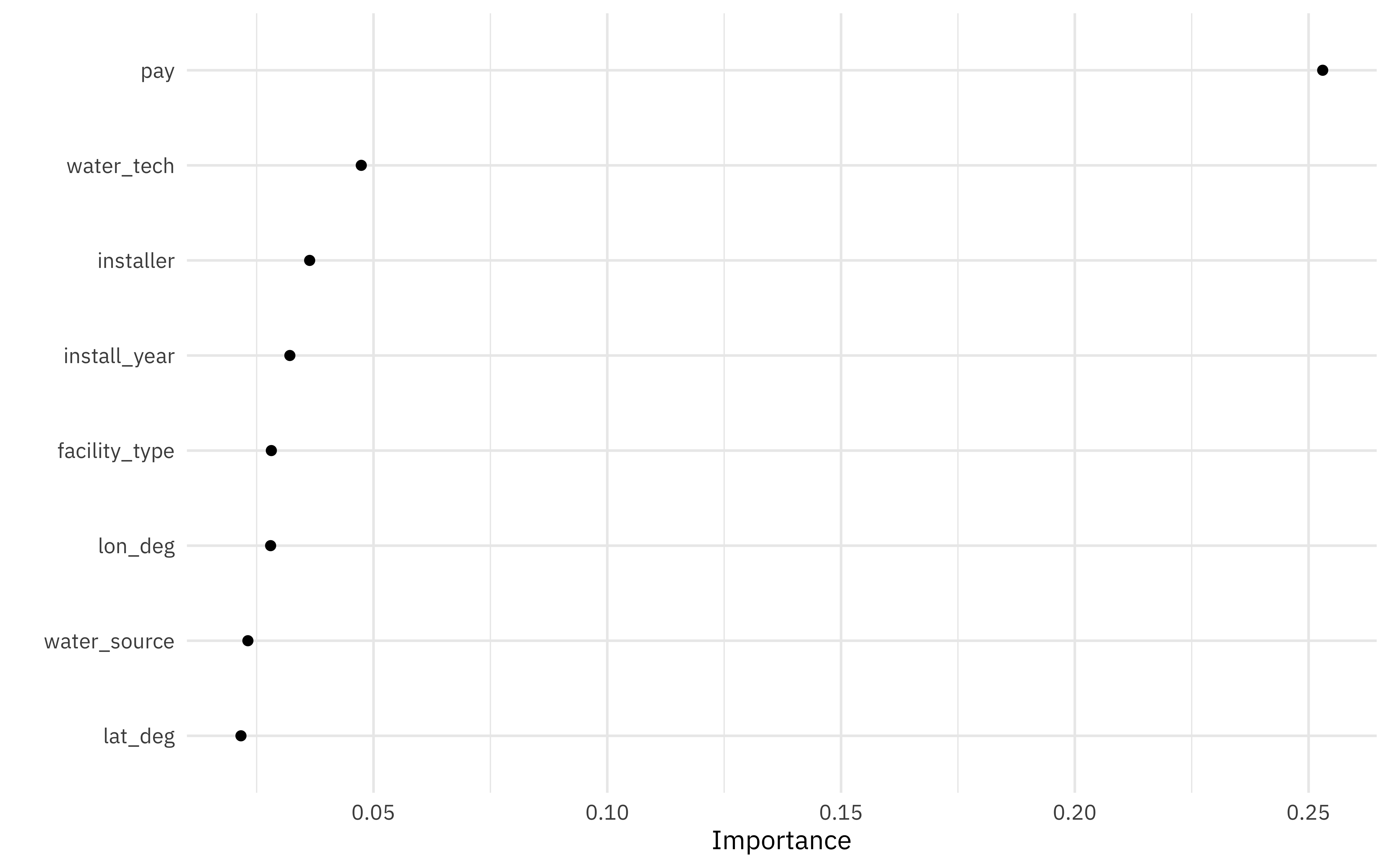
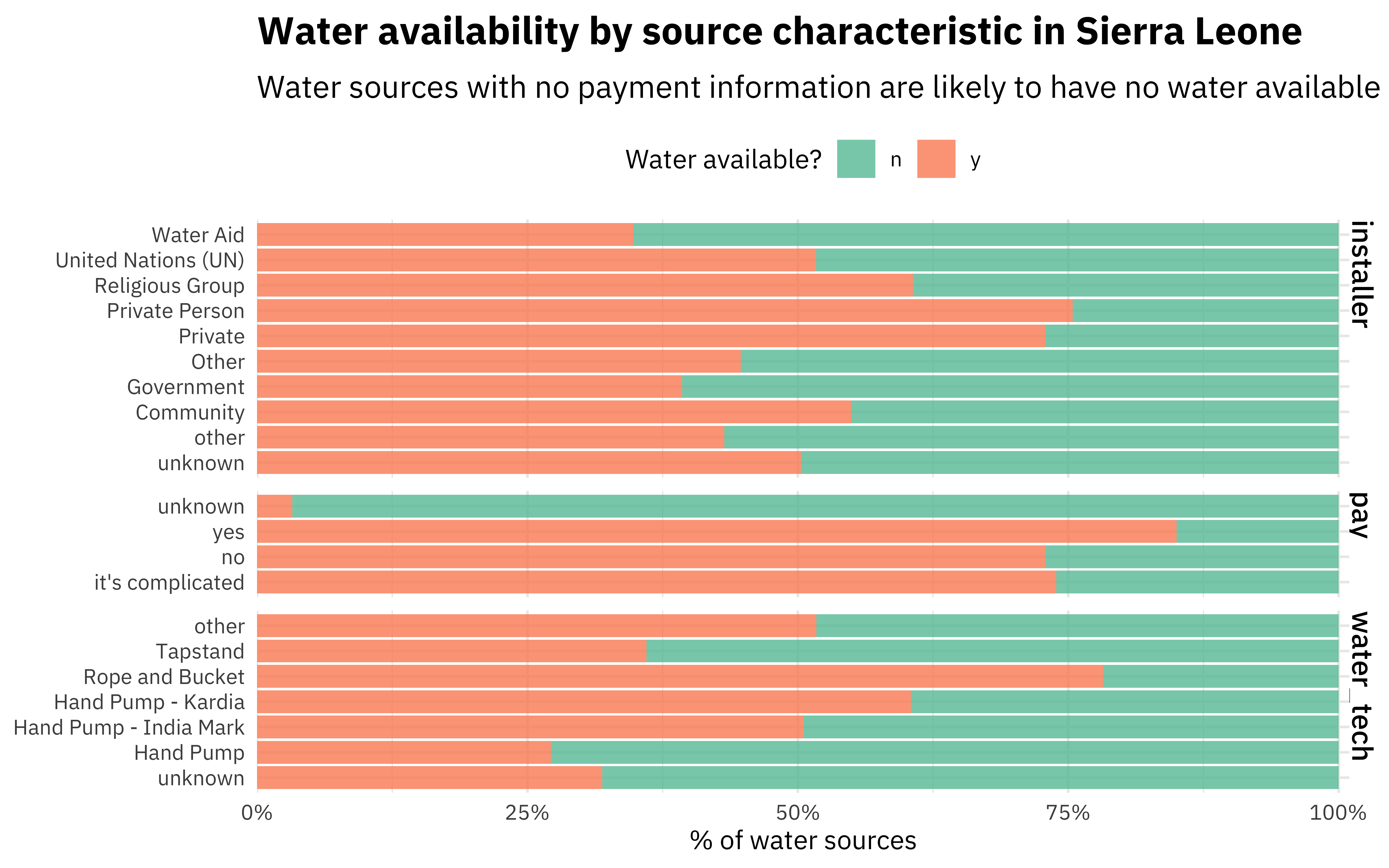
Not a huge surprise that pay is most important! The next most important variables are the technology used at the water source and who installed it. Let’s make one more plot using our preprocessed data to see how those are distributed.
imp_data %>%
  select(status_id, pay, water_tech, installer) %>%
  pivot_longer(pay:installer, names_to = "feature", values_to = "value") %>%
  ggplot(aes(y = value, fill = status_id)) +
  geom_bar(position = "fill") +
  facet_grid(rows = vars(feature), scales = "free_y", space = "free_y") +
  theme(legend.position = "top") +
  scale_fill_brewer(type = "qual", palette = 7) +
  scale_x_continuous(expand = expansion(mult = c(0, .01)), labels = scales::percent) +
  labs(
    x = "% of water sources", y = NULL, fill = "Water available?",
    title = "Water availability by source characteristic in Sierra Leone",
    subtitle = "Water sources with no payment information are likely to have no water available"
  )
- Posted on:
- May 6, 2021
- Length:
- 5 minute read, 983 words
- Categories:
- rstats tidymodels
- Tags:
- rstats tidymodels